flowchart LR
    A[Stats and Prob] --> B[Descriptive Statistics]
    A --> C[Distribtuions]
    A --> D[Population Inference]

    E[Data Exploration] --> F[Plotting]
    E --> G[Dataframes]
    E --> H[Exploratory Data Analysis]
CISC482 - Lecture17
Supervised Learning - KNN
Dr. Jeremy Castagno
Class Business
Schedule
Today
- Review Exam Results
- Introduction to Supervised Learning
- KNN
Exam Review
Exam Results
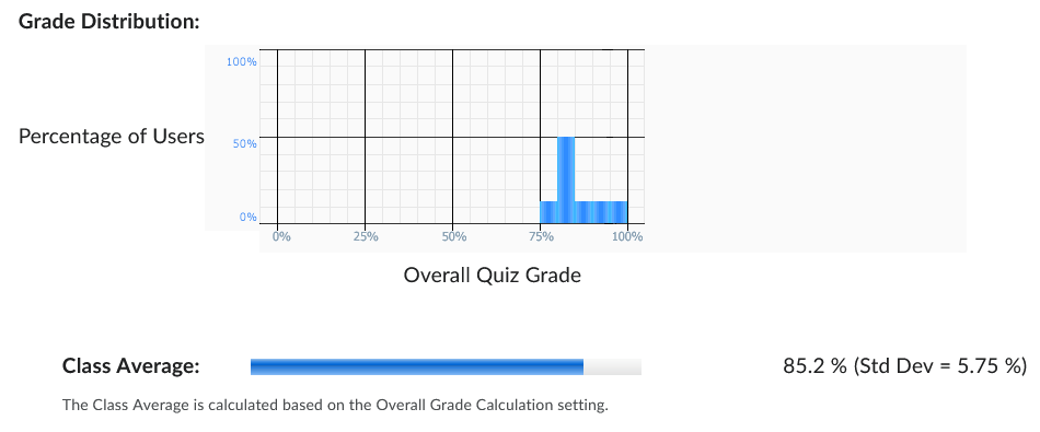
- Curve: +3 Bonus Points (3 questions, 6% bump)
- Average: 85%
Top Difficult Questions - #1
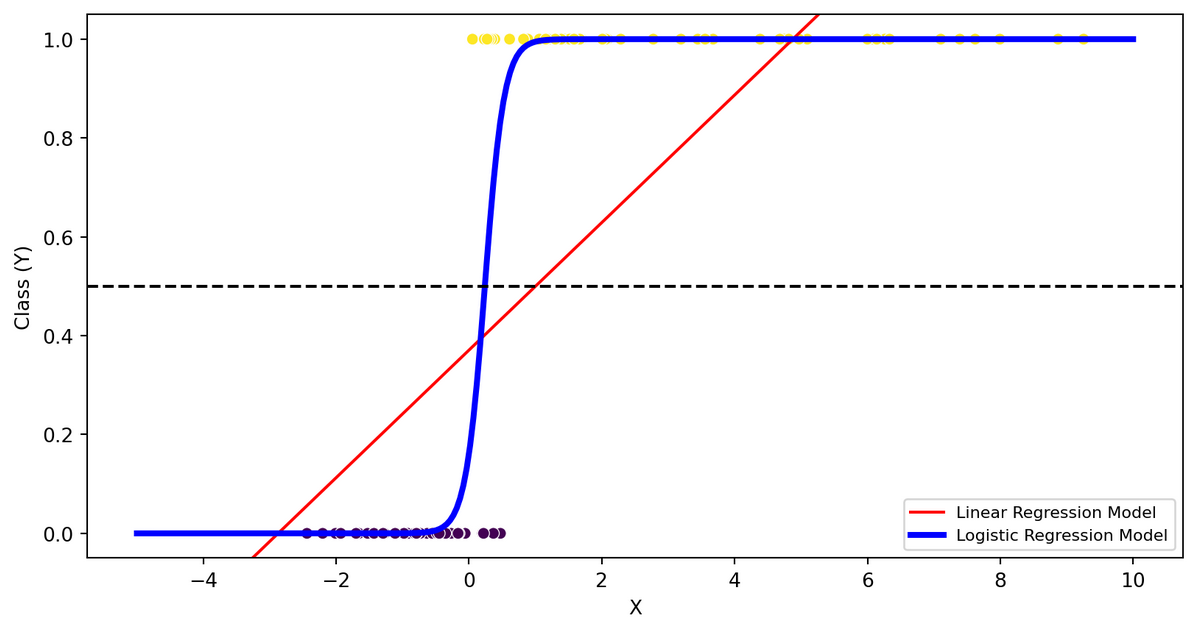
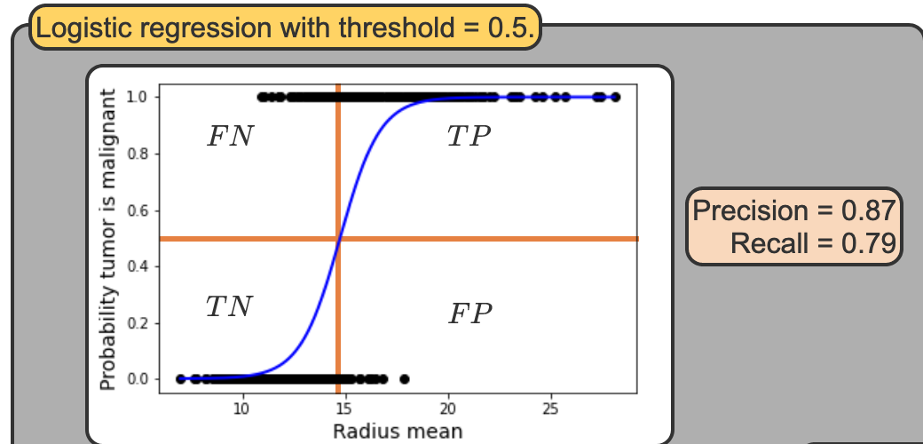
- Linear model has higher precision
- Linear model has worse recall
- Linear model has more FP
- Linear model has more FN
FN, TP, TN, FP
Top Difficult Questions - #2
Select all non-linear functions with respect to model parameters \(\mathbf{\beta}\)
- \(\beta_0 sin(x)\)
- \(\beta_0 x^2\)
- \(\frac{e^{\beta_0 + \beta_1 x}}{1 + e^{\beta_0 + \beta_1 x}}\)
- \(e^{\beta_0 + \beta_1 x}\)
- \(sin(\beta_0 x)\)
Top Difficult Questions - #3
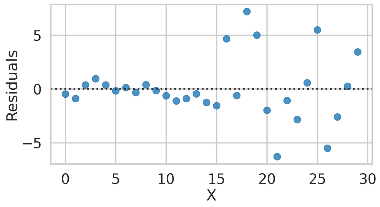
- Please explain if the assumptions of Linear Regression are met or not.
- You must discuss at least 3 of the assumptions and clearly explain if each assumption is met from looking at the graph.
Top Difficult Questions - #4
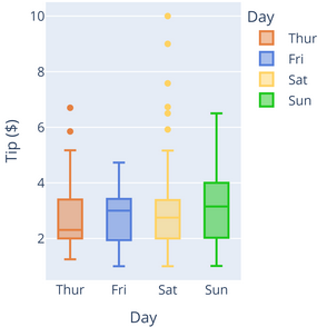
- Which day had the largest tip?
Big Picture
First 1/4
First 1/2
flowchart LR
    A[Regression] --> B[Linear Regression]
    A --> C[Mutliple Linear Regression]
    A --> D[Polynomial Regression]
    A --> Z[Logistic Regression]

    E[Model Evaluation] --> F[RMSE, R^2]
    E --> G[Precision, Recall]
    E --> H[Train,Valid,Test ]
Whats next
- More advanced models!
- We will still be using what we learned! Especially model evaluation!
- Fully define concept of supervised learning
Supervised Learning
Terms
- An instance is labeled if the outcome feature’s value is known for that instance.
- Supervised learning is training a model to predict a labeled outcome feature based on input features.
- The outcome feature is also known as the target or dependent variable.
- The input features are also known as features or independent variables
Example Regression Problem
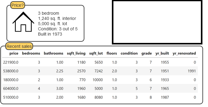
Example Classification Problem

Regression vs Classification
- Regression - Predicting a continuous numeric outcome
- Classification - Predicting the class (group) of an instance
Goals of Supervised Learning
Predict the values that unlabeled data will have and to explain how the inputs lead to the predicted outputs.
A model is interpretable if the relationship between input and output features in the model are easy to explain.
A model is predictive if the outcomes produced by the model match the actual outcomes with new data.
What is more important
- A model can be both predictive and interpretable, but different clients and disciplines value one more than the other.
- Ex: Scientists value interpretability more to explain the effect of experiments; image recognition models value predictiveness more.
- A large business may really only care about results. Being predictive may be the only thing that matters
K-nearest Neighbors (KNN)
Introduction
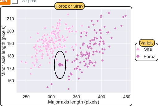
- k-nearest neighbors (kNN) is a supervised learning algorithm that predicts the output feature of a new instance using other instances that are close for certain input features.
- A value of k is selected and the k instances with the closest input features are found. The output features of those k instances are used to make the prediction.
Tip
Sometimes, the phrase “birds of a feather flock together” is used to describe the k-nearest algorithm, meaning the algorithm assumes that instances with similar inputs will have similar outputs.
Motivation
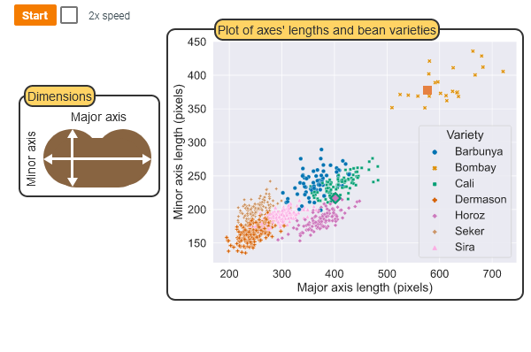
Example
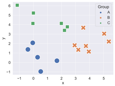
- (4, 2.5)
- (0, 4)
- (2, 1)
Finding your nearest neighbors
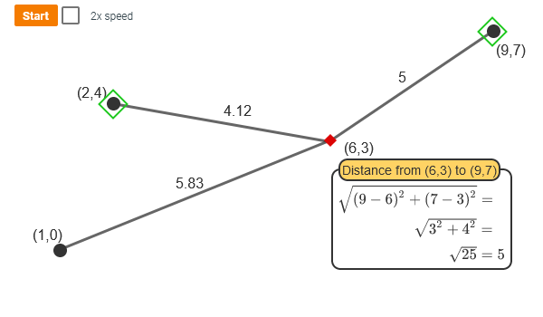
- How do determine how close a point is form the another (metric)
- distance(x,y) = \(\sqrt{(x_1 - y_1)^2 + (x_2 - y_2)^2 + ... + (x_p - y_p)^2 }\)
![Distance Calculation]()
Using KNN for Classification
Regression with KNN
- Select k, the number of neighbors to consider.
- Calculate the distance between all labeled instances and the instance to predict.
- The k instances with the shortest distances are the nearest neighbors.
- Predict by averaging the k nearest neighbors’ output values.
Software
scikit-learn
- KNeighborsClassifier
- KNeighborsClassifier
- Very easy to use! Lets do an example
Example - Data
Code
X, y = make_blobs(n_samples=100, centers=2, cluster_std=1.5, n_features=2,
                  random_state=0)
c_names = ["Class 0", "Class 1"]
fig, ax = plt.subplots(nrows=1, ncols=1)
scatter = ax.scatter(X[:, 0], X[:, 1], c=y, cmap='viridis');
ax.legend(handles=scatter.legend_elements()[0],
           labels=c_names,
           title="Class")
<matplotlib.legend.Legend at 0x7f12d8dd24d0>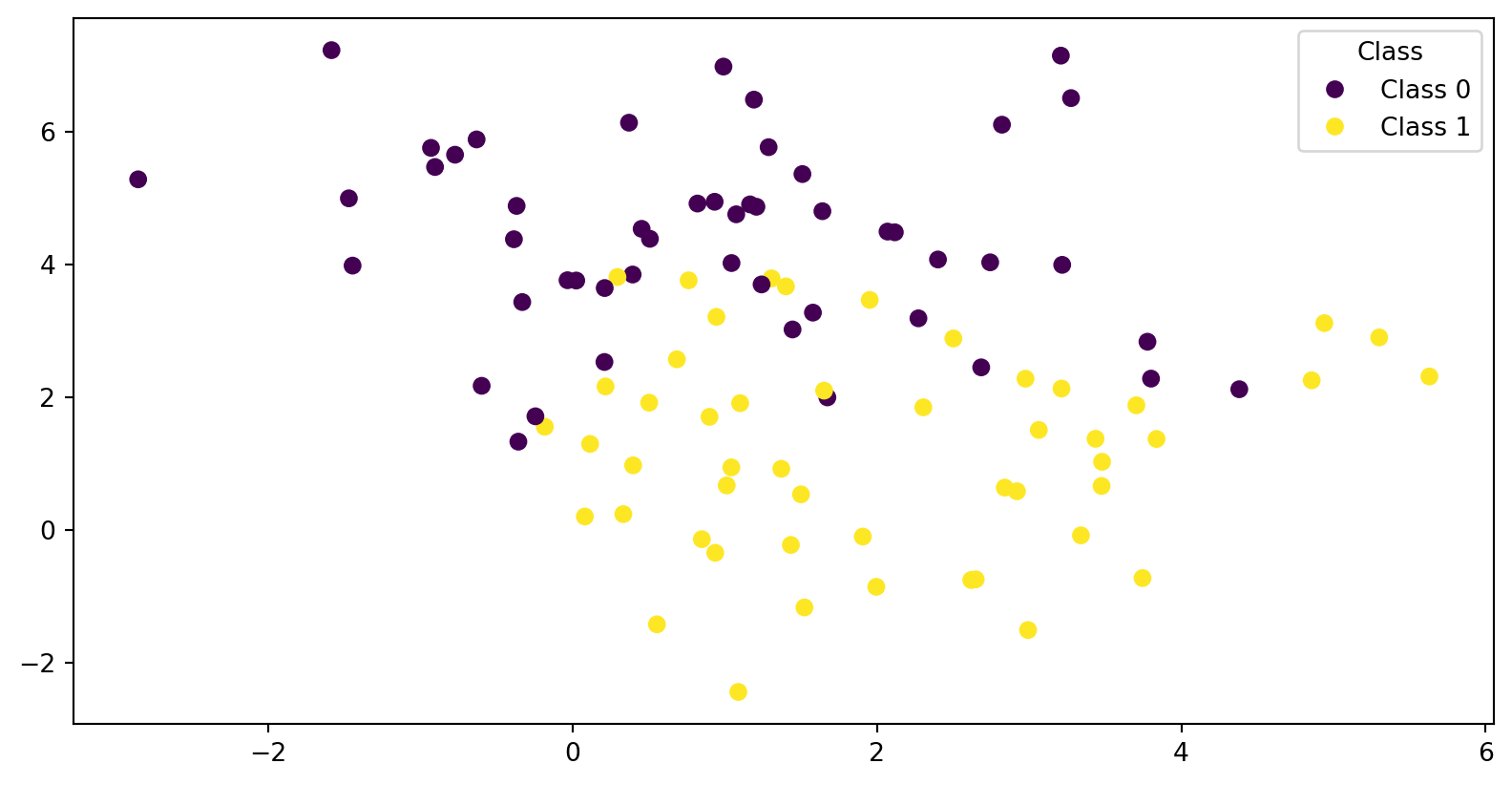
Split into Train and Test
Code
from sklearn.model_selection import train_test_split
# Split data
X_train, X_test, y_train, y_test = train_test_split(X, y, test_size=0.30, random_state=0)

# Plot data
fig, ax = plt.subplots(nrows=1, ncols=2)

data = [(X_train, y_train, 'Train Set'), (X_test, y_test, 'Test Set')]
for (X, y, title), ax_ in zip(data, ax):
  scatter = ax_.scatter(X[:, 0], X[:, 1], c=y, cmap='viridis')
  ax_.set_title(title)
  ax_.set_xlabel("X0")
  ax_.set_ylabel("X1")
  ax_.legend(handles=scatter.legend_elements()[0],
           labels=c_names,
           title="Class")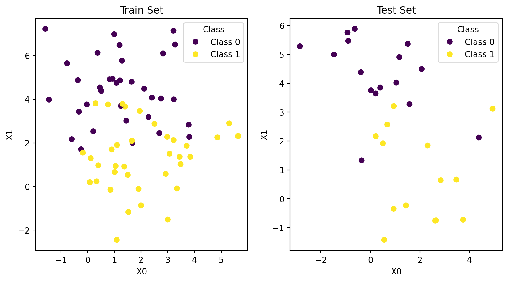
Train Model, Sanity Check
Code
from sklearn.neighbors import KNeighborsClassifier
# Create and train model
model = KNeighborsClassifier(n_neighbors=5)
model.fit(X_train, y_train)

# Single point sanity check
test_point = [2, 1]
predicted_group = model.predict([test_point])
print(f"We predict that {test_point} will belong to class: {predicted_group}")
We predict that [2, 1] will belong to class: [1]Test Model
Code
# Make predictions
predictions = model.predict(X_test)

# Plot data
fig, ax = plt.subplots(nrows=1, ncols=2)
data = [(X_test, y_test, 'Test Set (Ground Truth)'), (X_test, predictions, 'Test Set Predicted')]
for (X, y, title), ax_ in zip(data, ax):
  scatter = ax_.scatter(X[:, 0], X[:, 1], c=y, cmap='viridis')
  ax_.set_title(title)
  ax_.set_xlabel("X0")
  ax_.set_ylabel("X1")
  ax_.legend(handles=scatter.legend_elements()[0],
           labels=c_names,
           title="Class")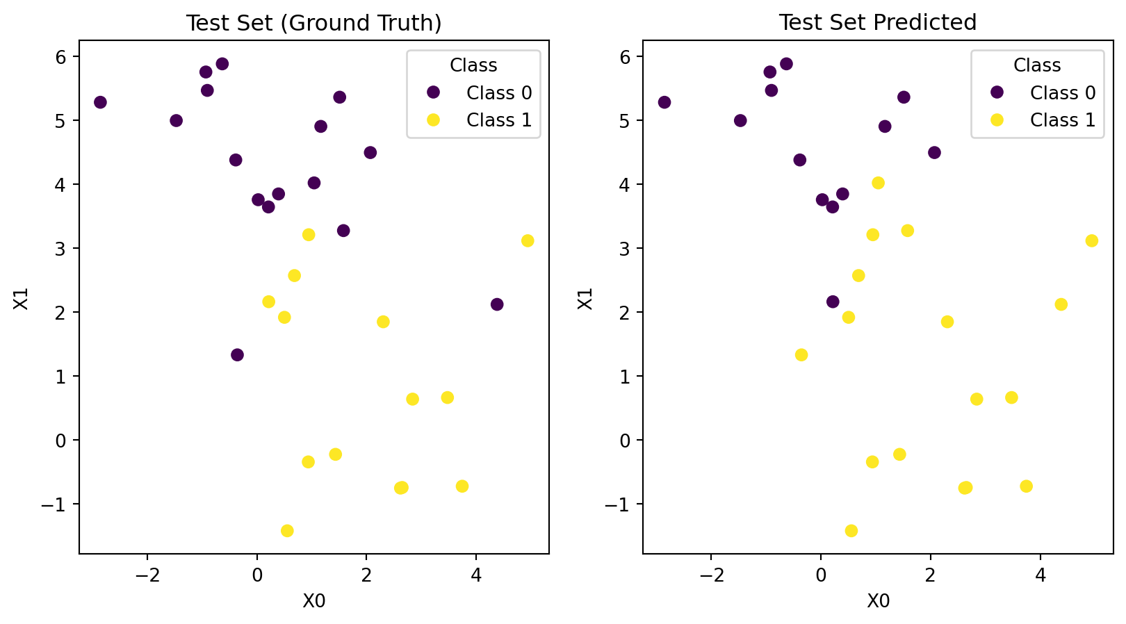
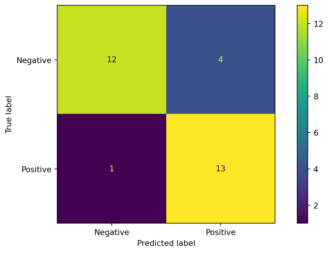
Confusion Matrix, Plot
Classication Metrics
- Accuracy = \(\frac{TP+TN}{TP+TN+FP+FN}\)
- Precision = \(\frac{TP}{TP+FP}\)
- Recall = \(\frac{TP}{TP+FN}\)
- F1 = \(\frac{2*Precision*Recall}{Precision+Recall} = \frac{2*TP}{2*TP+FP+FN}\)
Classification Report
Code
              precision    recall  f1-score   support

    Negative       0.92      0.75      0.83        16
     Postive       0.76      0.93      0.84        14

    accuracy                           0.83        30
   macro avg       0.84      0.84      0.83        30
weighted avg       0.85      0.83      0.83        30
