CISC482 - Lecture14
Evaluating Model Performance 1
Class Business
Schedule
- Reading 6-1: Mar 08 @ 12PM, Wednesday
- Reading 6-2: Mar 10 @ 12PM, Friday
- Proposal: Mar 22, Wednesday
- HW5 - Mar 29 @ Midnight, Wednesday
Today
- Overfit/Underfit
- Bias/Variance Trade off
- Regression Metric
- Binary Classification Metrics
Model Error
Modelling
- We approximate an output feature \(y\), using input features \(X\) with function \(f\) such that \(\hat{y} = f(X)\)
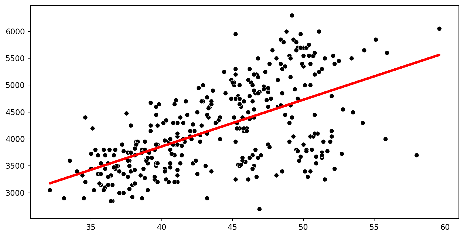
- Example: Predicting penguin body mass by bill length
- \(\text{body mass} = \hat{y} = mx + b\)
- We have to choose \(f\) and \(X\): simple linear model, polynomial model, multiple linear regression, logistic regression, etc.
- Example is \(\hat{y} = \beta_0 + \beta_1 x\) or is \(\hat{y} = \beta_0 + \beta_1 x + \beta_2 x^2\)
Underfit
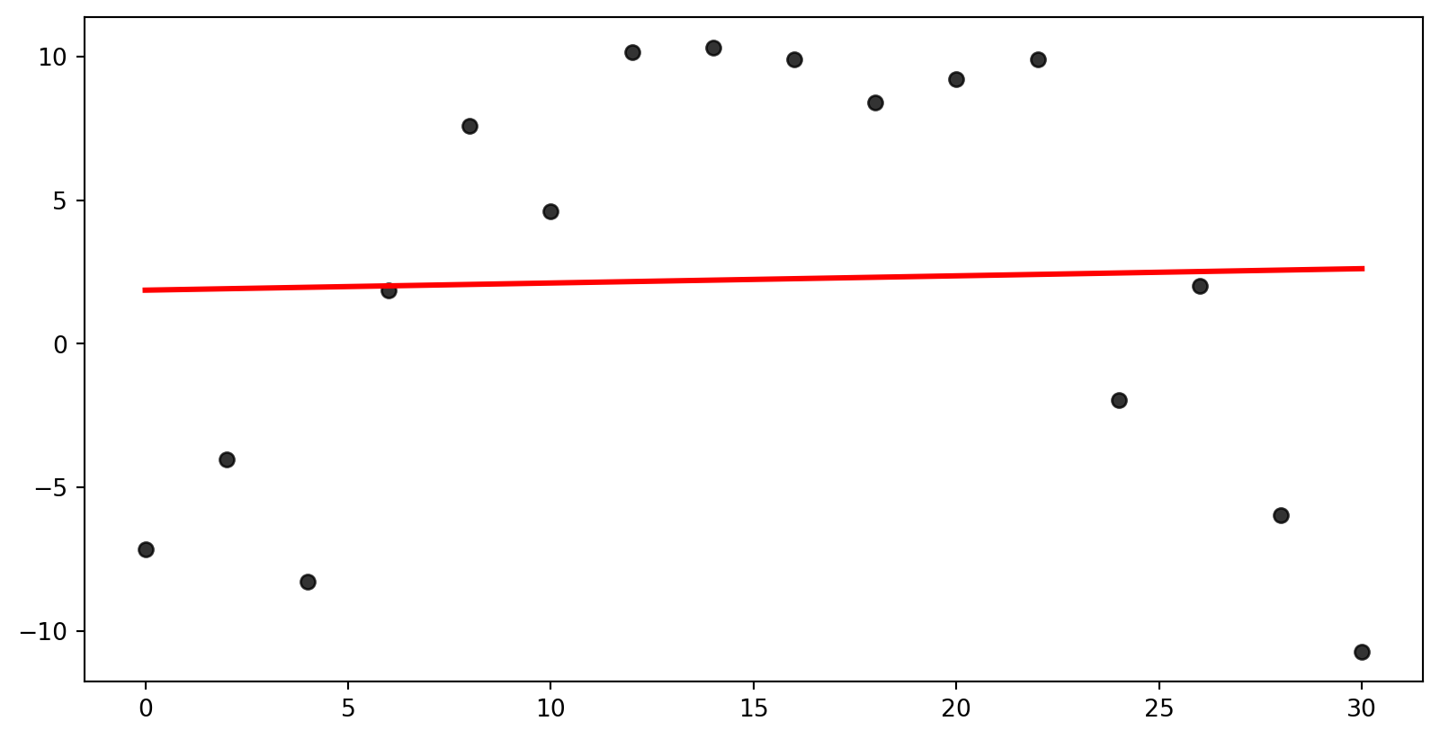
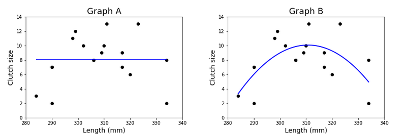
- Underfit - model is too simple to fit the data well.
Underfit Problems
- An underfit model will miss the underlying trend
- Will score poorly in metrics
Overfit
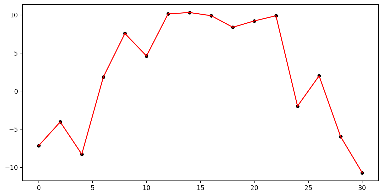
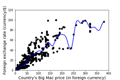
- Overfit - model is too complex to fit the data well.
Overfit Problems
- Fitting the data too closely
- Incorporating too much noise (meaningless variation)
- Misses the general trend of the data despite scoring well in some metrics
- In fact, what is the error for this model?
Optimal
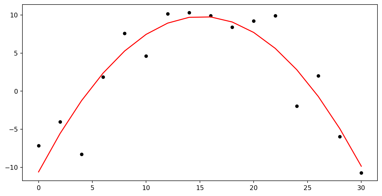
- This model would be best fit with a quadratic model
Note
Important
A model that is overfit or underfit is a bad predictor of outcomes outside of the data set and should not be used. In the field of data science, models tend to be overfit, so model selection techniques focus on choosing the least complex model that captures the general trend.
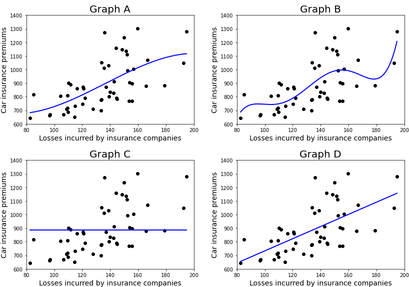
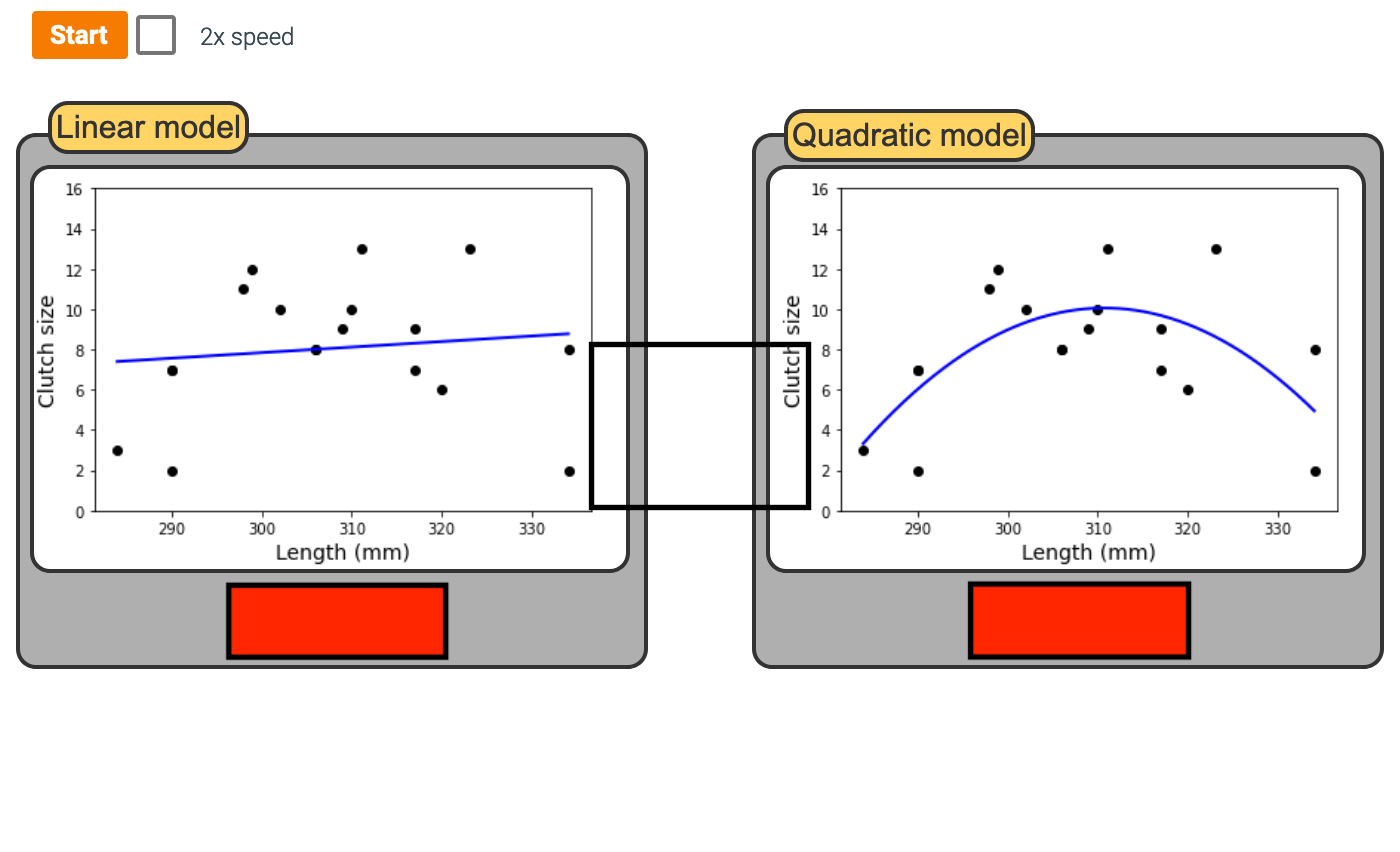
Find Most Underfit and Most Overfit
Bias and Variance
Breaking down Error
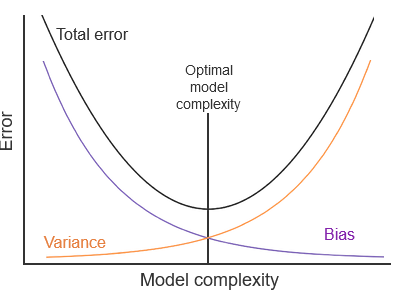
- The total error of a model is how much the observed values differ from predicted values. Total error is broken down into three pieces:
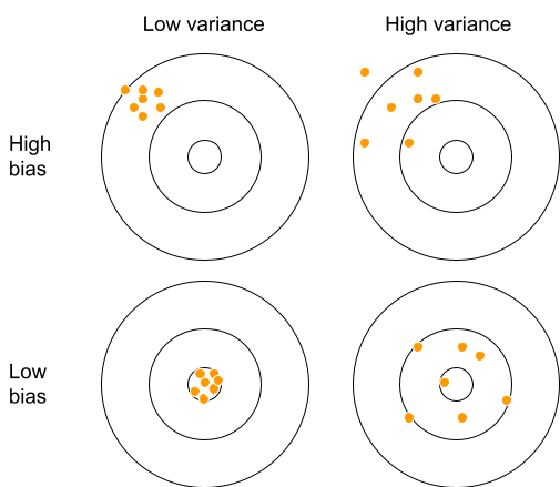
- Bias - model’s prediction differs from the observed values due to the assumptions built into the model.
- Variance - spread/variance of predictions
- Irreducible error - error inherent to the data (noise)
Visual Explanation
Bias-Variance Tradeoff
- Choosing a more complex model (more features, a more complicated mathematical expression, etc.) means the model’s predictions are closer to the observed sample values, which decreases the bias.
- However, doing so makes the model’s predictions more spread out to meet the observed values, increasing the variance.
- An optimal model should be just complex enough to capture the general trend of the data (low bias) without incorporating too much of the noise from the sample (low variance).
Visual Example
Problem 1
Problem 2
Regression Metrics
Dataset
- We will be using the penguin dataset
| species | island | bill_length_mm | bill_depth_mm | flipper_length_mm | body_mass_g | sex | year | |
|---|---|---|---|---|---|---|---|---|
| 0 | Adelie | Torgersen | 39.10 | 18.70 | 181.00 | 3,750.00 | male | 2007 |
| 1 | Adelie | Torgersen | 39.50 | 17.40 | 186.00 | 3,800.00 | female | 2007 |
| 2 | Adelie | Torgersen | 40.30 | 18.00 | 195.00 | 3,250.00 | female | 2007 |
| 4 | Adelie | Torgersen | 36.70 | 19.30 | 193.00 | 3,450.00 | female | 2007 |
| 5 | Adelie | Torgersen | 39.30 | 20.60 | 190.00 | 3,650.00 | male | 2007 |
Two statistics
R-squared, \(R^2\) : Percentage of variability in the outcome explained by the regression model (in the context of SLR, the predictor)
\[ R^2 = \frac{\text{variation explained by regression}}{\text{total variation in the data}} = \frac{\sum (\hat{y}_i - \bar{y})^2}{\sum (y_i - \bar{y})^2} \\ R^2 = 1 - \frac{\sum (\hat{y}_i - y_i)}{\sum (y_i - \bar{y})^2} \]
Root mean square error, RMSE: A measure of the average error (average difference between observed and predicted values of the outcome)
\[ RMSE = \sqrt{\frac{\sum_{i = 1}^n (y_i - \hat{y}_i)^2}{n}} \]
What indicates a good model fit? Higher or lower \(R^2\)? Higher or lower RMSE?
R-squared
- Ranges between 0 (terrible predictor) and 1 (perfect predictor), Unitless
- Calculate with
model.score(X, y):
More Examples
Graph
\(R^2\) Example
Interpreting R-squared
The \(R^2\) of the model for predicting penguin mass from bill length is 25%. Which of the following is the correct interpretation of this value?
- Bill Length correctly predicts 25% of penguin mass.
- 25% of the variability in penguin mass can be explained by bill length.
- 25% of the time penugin mass can be predicted by bill length.
RMSE
Ranges between 0 (perfect predictor) and infinity (terrible predictor)
Same units as the outcome variable
Calculate with
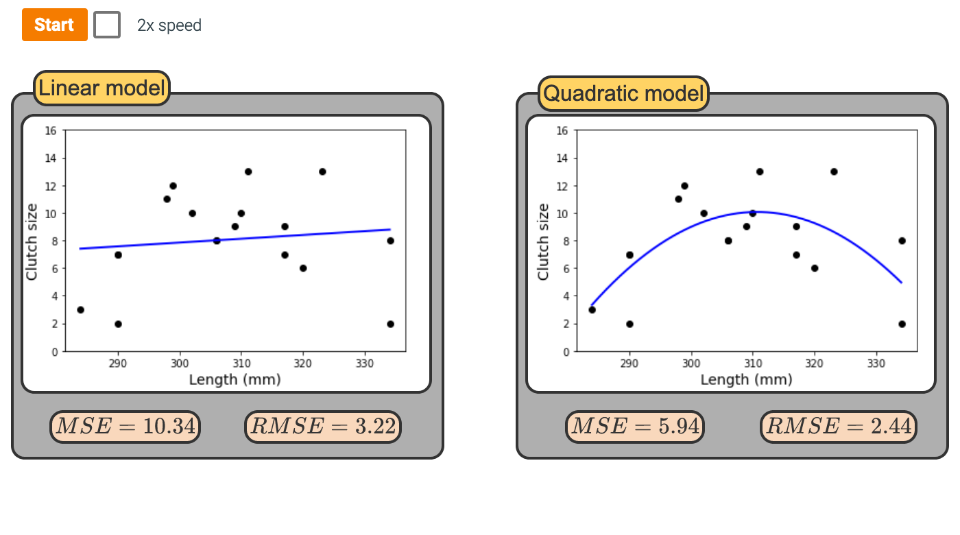
means_squared_error(y_true, y_pred):The value of RMSE is not very meaningful on its own, but it’s useful for comparing across models.
Comparing a model that uses bill length for a predictor or using flipper length
RMSE Example
Binary Classification Metrics
True/False Positive/Negative
- True Positive (TP) is an outcome that was correctly identified as positive
- True Negative (TN) is an outcome that was correctly identified as negative.
- False Positive (FP) is an outcome that was incorrectly identified as positive
- False Negative (TN) is an outcome that was incorrectly identified as negative
Confustion Matrix
| Positive (predicted) | Negative (predicted) | |
|---|---|---|
| Positive (actual) | 170 | 21 |
| Negative (actual) | 1 | 377 |
Metrics
- Accuracy - useful
- Precison - very useful
- Recall - very useful
Accuracy
- Accuracy: \(\frac{\text{# Correctly Predicted}}{\text{Total}}\)
- \(\frac{TP + TN}{TP + TN + FP + FN}\)
Precision
- Tell how precise your prediction is
- \(\frac{TP}{TP + FP}\)
- The higher this number, the less False Positives you have
- My research - Identifying an emegency landing location nearby. A precison gives confidence that it truly is safe to land at the location the model predicts.
Recall
- the proportion of positives that were correctly predicted
- \(\frac{TP}{TP + FN}\)
- The higher this number, the less False Negative you have.
- My Research - A high recall means I found nearly all the rooftops in the city that you could land on.
Example Question
| Positive (predicted) | Negative (predicted) | |
|---|---|---|
| Positive (actual) | 170 | 21 |
| Negative (actual) | 1 | 377 |
What is the Accuracy, Precision, and Recall?
Tradeoff Between Precision and Recall
Tradeoff
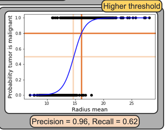
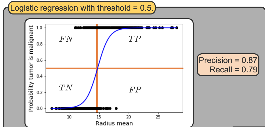
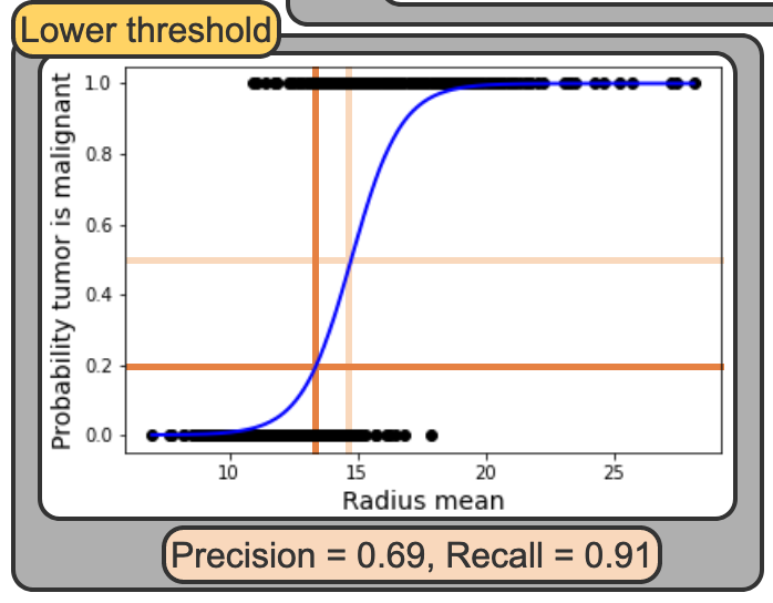
- In logisitc regression you specify a threshold to use a prediciton. By deafult we use 0.5 or 50%. But that is arbitary and you move that threshold
Low Threshold
High Threshold
