CISC482 - Lecture12

Logistic Regression

Dr. Jeremy Castagno

Class Business

Schedule

• Reading 6-1: Mar 08 @ 12PM, Wednesday
• Topic Ideas - Should be turned in! Will grade soon!
• HW4 - Mar 08 @ Midnight
• Proposal: Mar 22, Wednesday

Today

• Review Linear Regression
• Logistic Regression

Review Linear Regression

What we learned

• Simple Linear Regression
  • \(\hat{y} = \beta_0 + x + \beta_1\)
• Simple Polynomial Linear Regression
  • \(\hat{y} = \beta_0 + \beta_1 x + ... + \beta_k x^k\)
• Multiple Linear Regression
  • \(\hat{y} = \beta_0 + \beta_1 x_1 + ... \beta_k x_k\)
• Multiple (Variable) Polynomial Regression
  • \(\hat{y} = \beta_0 + \beta_1 x_1 + \beta_2 x_1^2 + \beta_3 x_1 x_2 + \beta_4 x_2 + \beta_5 x_2^2\)

Regression Diagram

flowchart LR
  A[Features] --> B{Single Feature}
  B -- Yes --> C{Curvature}
  C -- No --> E[Simple Regression]
  C -- Yes --> D[Simple Polynomial <br> Regression]
  B -- No --> F{Non-linear Correlation <br> Between Features}
  F -- No --> G[Multiple Linear <br> Regression]
  F -- Yes --> H[Polynomial Regression]

Class Activity

Class Activity

Demo!

Non Linear Regression

• Linear Regression - Linear Combination of features
  • \(\hat{y} = \beta_0 + \beta_1 x_1 + ... \beta_k x_k\)
• Parameters \(\beta_k\) are simply multiplied by features and added together
• Non-linear mathematical parameter’s with respect to \(\beta_k\)
• \(f(x, \beta)\)

Example Non Linear

• Trigonometric - \(sin(\beta_0 x)\)
• Exponential - \(e^{\beta_0 + \beta_1 x}\)
• Logistic - \(\frac{e^{\beta_0 + \beta_1 x}}{1 + e^{\beta_0 + \beta_1 x}}\)

Tip

This class will be focus on using logistic regression. But lets take a step back and talk about a new problem.

Classification

• We are now going to be focusing on problems where we are interested in predicting the group or the class of something
• Give \(X = {x_1, x_2, ..., x_k}\) what is the class of this object.
  • Given the bill_length is 10 and bill_depth is 20 what is the species of this penguin?
  • A person arrives at the emergency room with a set of symptoms. Which of the three medical conditions does the individual have?
• Lets first focus where there are only 2 classes. Lets just call them (+) positive and (-) negative.

Example Classification

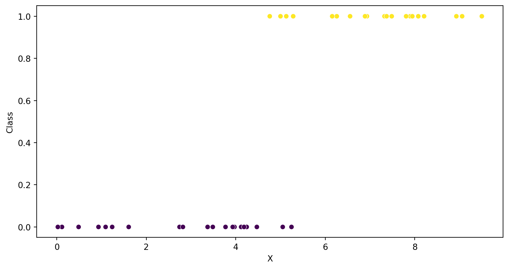
Linear Regression for Classification

• Linear Regression is generally not suitable for classification purposes
• However, you can use it to draw a line that whose value predicts the class
• E.g. if \(\hat{y} > 0.5 -> Positive\)

LR Classification (Okay)

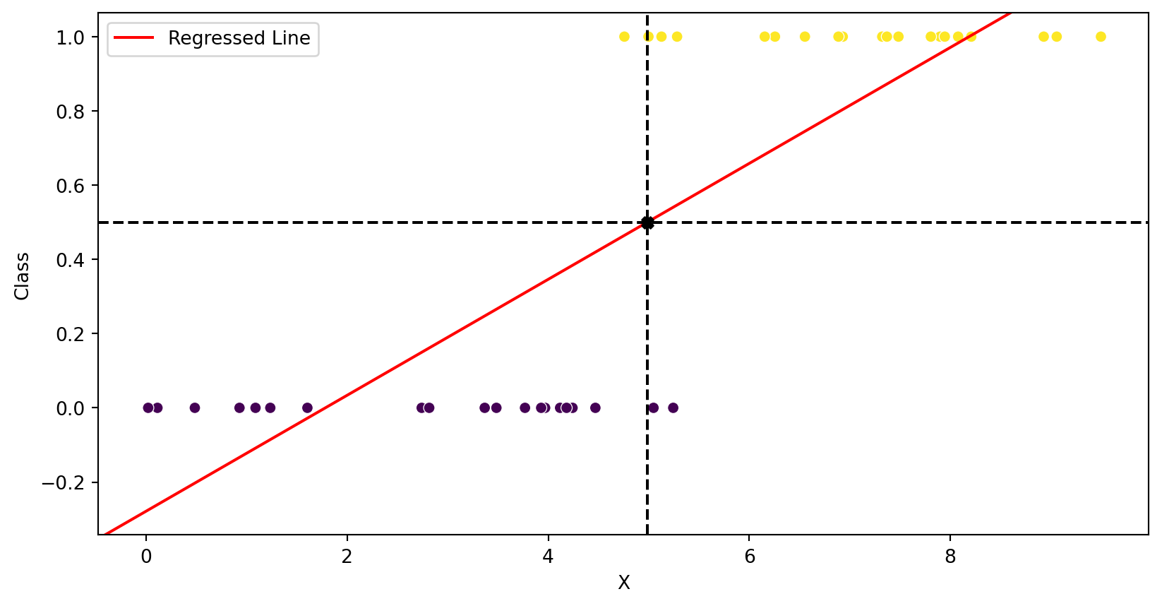
LR Classification (BAD)

LR Classification (Really BAD)

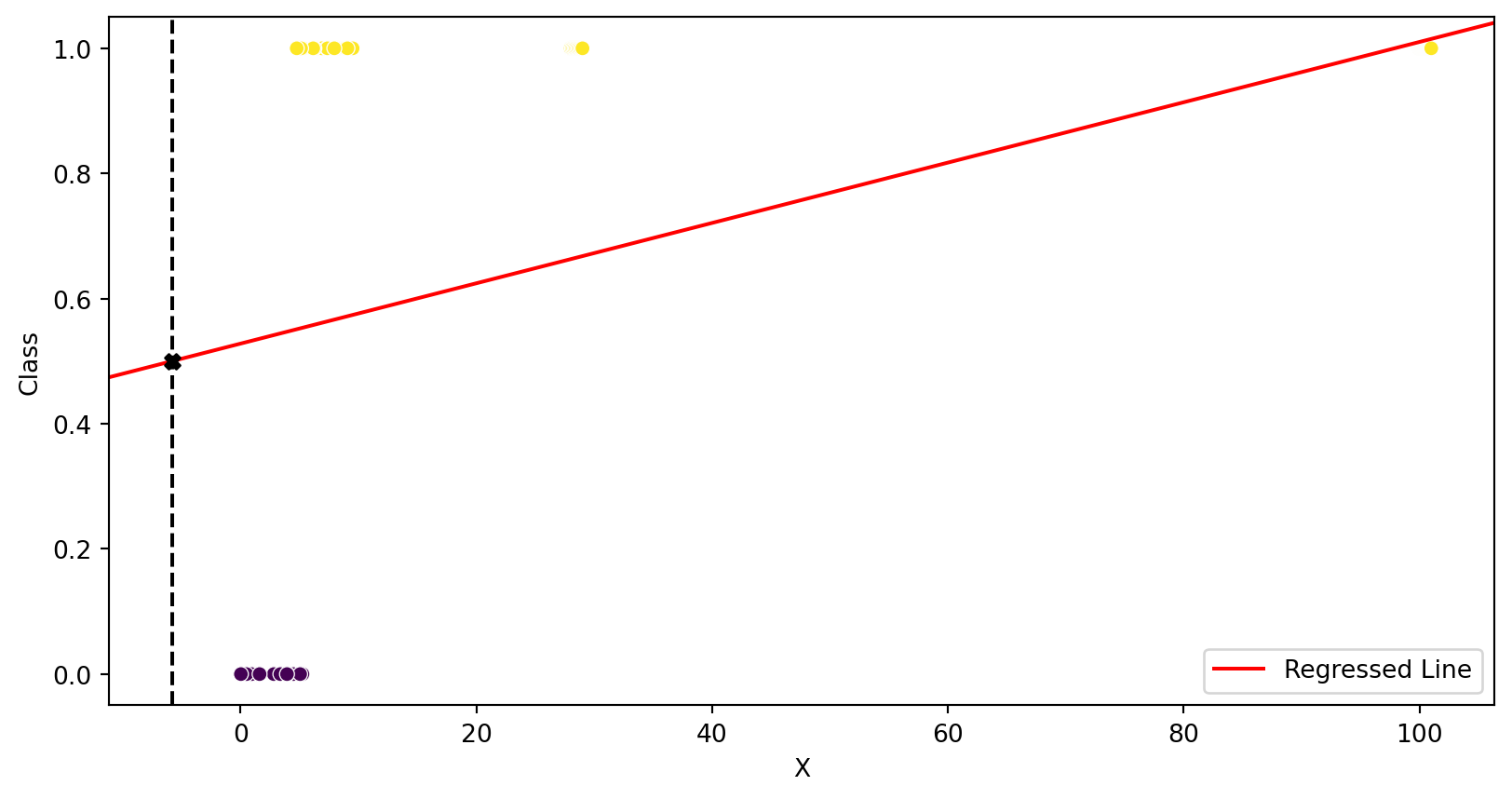
Logistic Regression

• Use a specific exponential function
• \(\hat{y} = \frac{e^{\beta_0 + \beta_1 x}}{1 + e^{\beta_0 + \beta_1 x}}\)
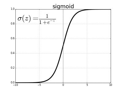
• Whats the range of this function?
• \(\hat{p} = \sigma(z)\), where
  • \(z = \beta_0 + \beta_1 x\)
  • \(\sigma(z) = \frac{e^{z}}{1 + e^{z}}\)
  • \(\sigma(z) = \frac{1}{1 + e^{-z}}\)

Example

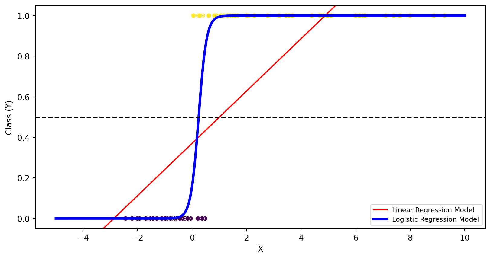
from sklearn.linear_model import LinearRegression, LogisticRegression

linear_model = LinearRegression()
logistic_model = LogisticRegression(C=1e5)

linear_model.fit(X, y)
logistic_model.fit(X, y)

print(f"LINEAR MODEL: {linear_model.coef_[0]:.1f} * x + {linear_model.intercept_:.1f}")
print(f"LOGISTIC MODEL: sigmoid({logistic_model.coef_[0][0]:.1f} * x + {logistic_model.intercept_[0]:.1f})");

LINEAR MODEL: 0.1 * x + 0.4
LOGISTIC MODEL: sigmoid(6.9 * x + -1.6)

Visual

Note

What do you notice?

Multivariable Classification

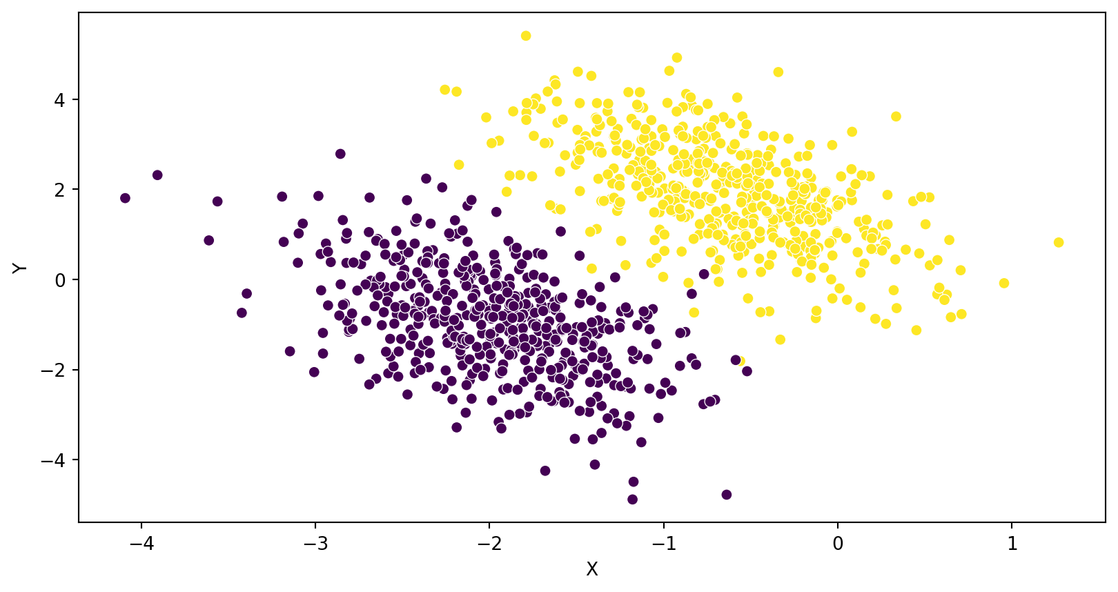
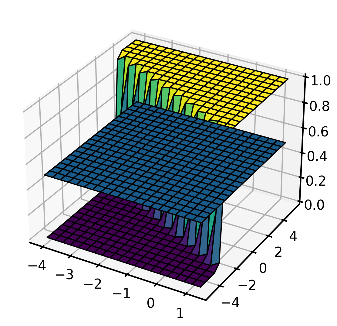
In 3D

Multivariable Logistic Regression

Code

logistic_model = LogisticRegression(C=1e5)
logistic_model.fit(X, y)

x_range = np.linspace(X[:, 0].min(), X[:, 0].max(), 20)
y_range = np.linspace(X[:, 1].min(), X[:, 1].max(), 20)
XX, YY = np.meshgrid(x_range, y_range)
P = expit(XX* logistic_model.coef_[0][0] + YY * logistic_model.coef_[0][0] + logistic_model.intercept_)


with sns.plotting_context("talk"):
  fig = plt.figure(figsize = (10, 7))
  ax = plt.axes(projection ="3d")
  # ZZ = np.ones_like(XX) * 0.5 
  # ax.plot_surface(XX, YY, ZZ,  **kwargs, zorder=1)
  ax.scatter(X[:,0], X[:,1], y, c=y, cmap='jet', zorder=10, edgecolor='k')
  ax.plot_surface(XX, YY, P, alpha=1.0, cmap='viridis', edgecolor='k');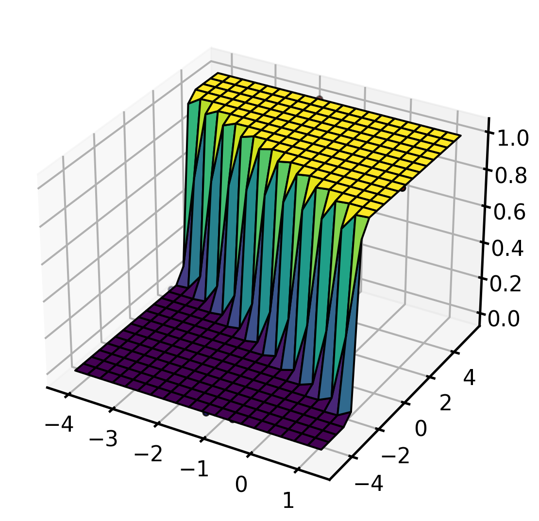

Multivariable Logistic Regression

Code

with sns.plotting_context("talk"):
  fig = plt.figure(figsize = (10, 7))
  ax = plt.axes(projection ="3d")
  ZZ = np.ones_like(XX) * 0.5 
  ax.plot_surface(XX, YY, ZZ,  zorder=1, edgecolor='k')
  ax.plot_surface(XX, YY, P, alpha=1.0, cmap='viridis', edgecolor='k');

View Decision Boundary

Code

from sklearn.inspection import DecisionBoundaryDisplay
disp = DecisionBoundaryDisplay.from_estimator(
    logistic_model, X, response_method="predict", cmap=plt.cm.viridis, alpha=0.5
)
disp.ax_.scatter(X[:,0], X[:,1], c=y, cmap='viridis', edgecolor='k');
disp.ax_.set_xlabel("X")
disp.ax_.set_ylabel("Y")

Text(0, 0.5, 'Y')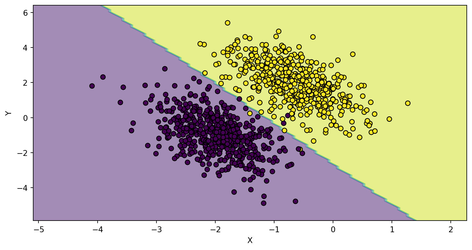

How it works

Loss Function

• Lets create a likelihood function \(L\) that is a function of our parameters \(\beta\). We want to find parameters \(\beta\) that make \(L\) as big as possible.
• \(L(\beta) = \sum_{i=1}^n \underbrace{y_i \cdot \sigma(\beta \; x_i)}_{y = 1} + \underbrace{(1-y_i) \cdot (1 - \sigma(\beta \; x_i))}_{y = 0}\)
• Convert to a loss function \(J\). We also take the logarithm. This ensures our cost function is convex.
• \(J(\beta) = -\sum_{i=1}^n y_i \cdot log(\sigma(\beta \; x_i)) + (1-y_i) \cdot log(\sigma(\beta \; x_i))\)
• This does not have a closed form solution. AKA you can not just take derivative and solve the parameters \(\beta\).
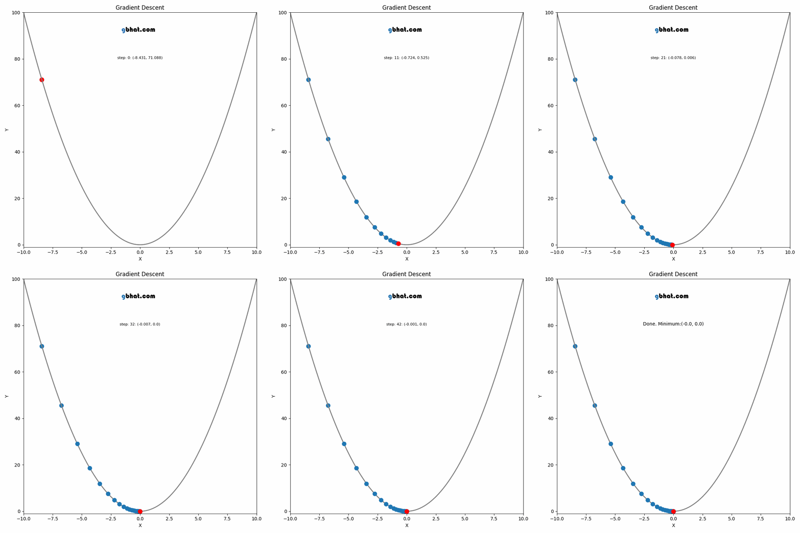
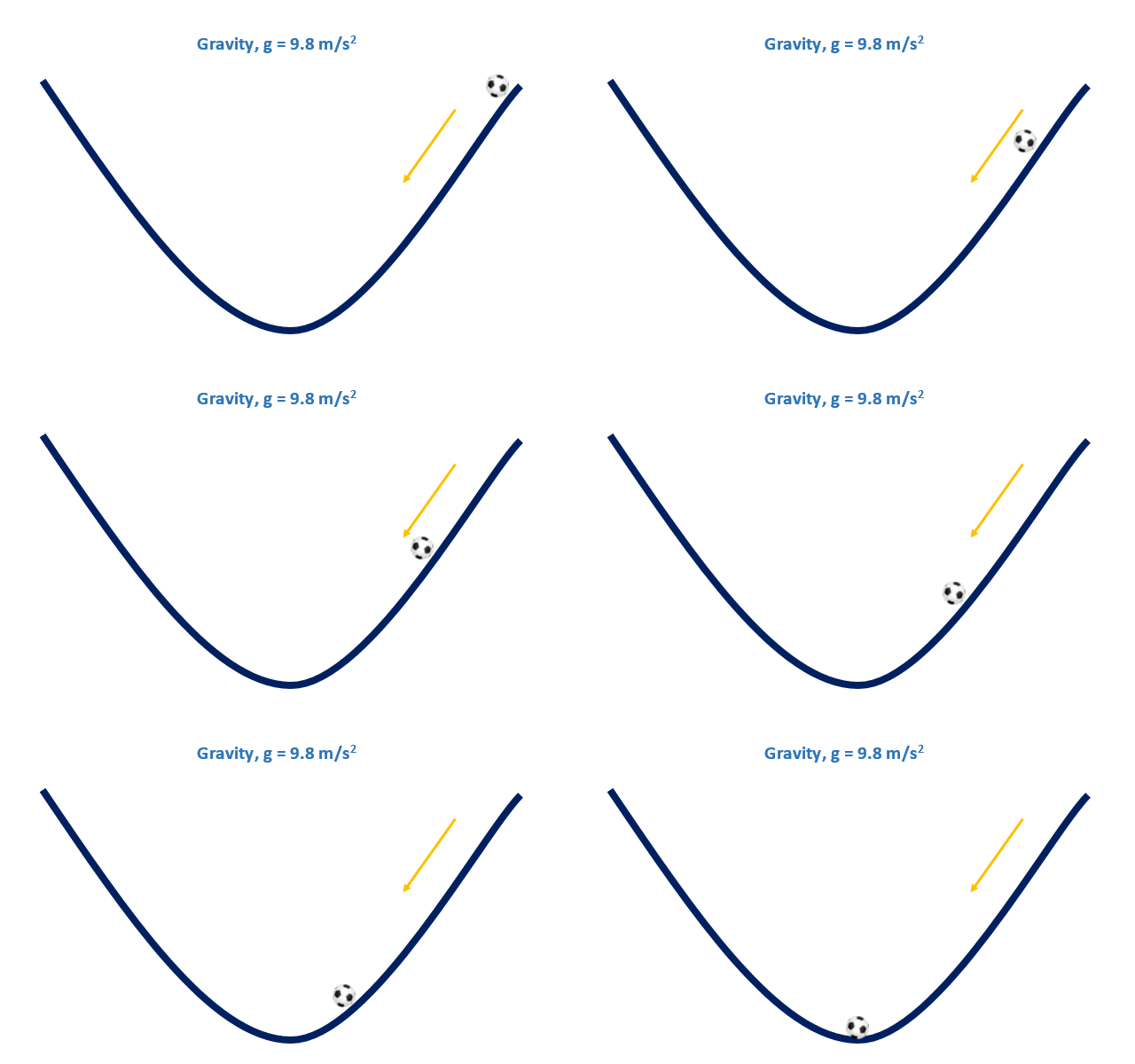
• We have to use a numerical solver. For example, gradient descent.

Convex vs Non Convex

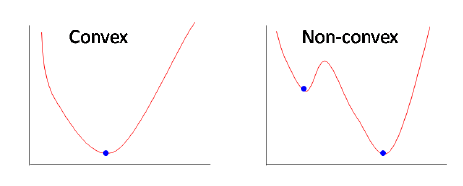
Convex Function, Soccer Ball

Gradient Descent