CISC482 - Lecture11

Regression 2

Dr. Jeremy Castagno

Class Business

Schedule

Topic Ideas - Should be turned in! Will grade soon!
Reading 5-3: Mar 01 @ 12PM, Wednesday
HW4 - Mar 08 @ Midnight
Proposal: Mar 22, Wednesday

Today

Assumptions of Linear Regression
Multiple Linear Regression

Review

Review Simple Linear Regression

What is the model for linear regresion: \(\hat{y} = ?\)
What is residual?
What is the loss function to solve for the parameters
- \(L(\beta_0, \beta_1) = \sum\limits_{i=1}^{n}[y_i - \hat{y}_i]^2\)
- \(L(\beta_0, \beta_1) = [y_i - (\hat{\beta}_0 + \hat{\beta}_1 x_i)]^2\)

Formulas?

\(\beta_1 (slope) = \frac{\sum\limits_{i=1}^{n}[(x_i-\bar{x})(y_i- \bar{y})]}{\sum\limits_{i=1}^{n} (x_i - \bar{x})^2}\)

\(\beta_0\) (intercept) = \(\bar{y} - \beta_1 \bar{x}\)

\(\hat{\beta}_1 (slope) = \frac{\text{Cov}(x,y)}{s_x^2} = r\frac{s_y}{s_x}\)

\(\beta_0\) (intercept) = \(\bar{y} - \beta_1 \bar{x}\)

Assumptions

Assumptions of Linear Regression

\(x\) and \(y\) have a linear relationship.
The residuals of the observations are independent.
The mean of the residuals is 0 and the variance of the residuals is constant.
The residuals are approximately normally distributed.

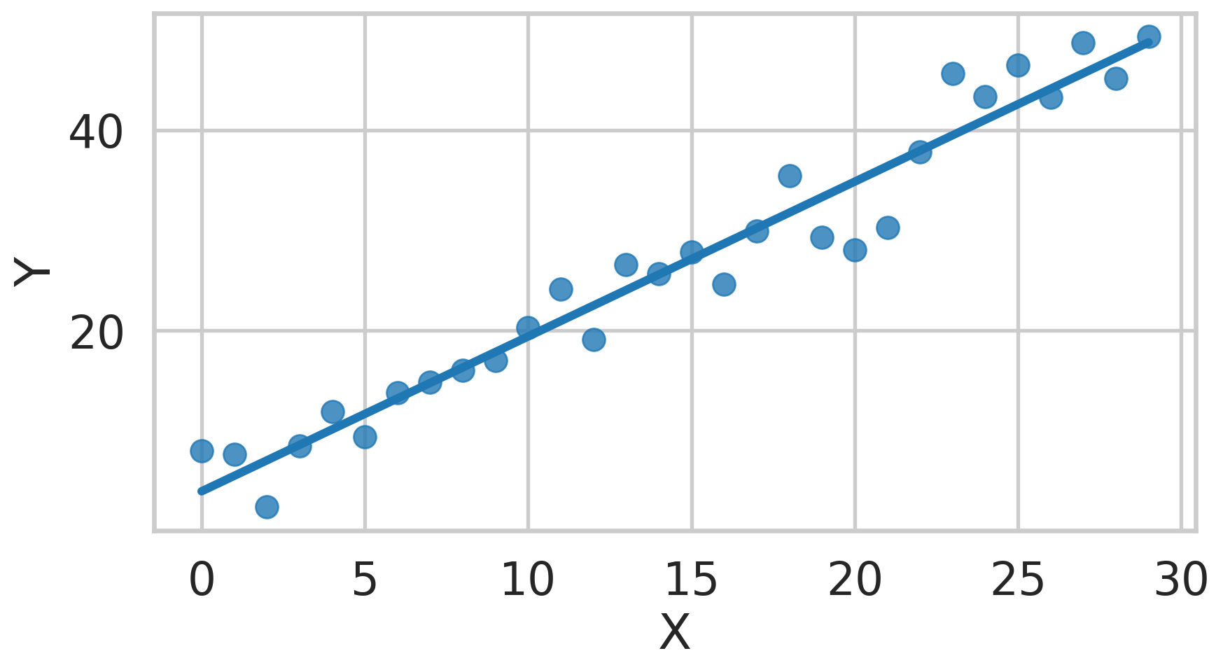
Linear Relationship?

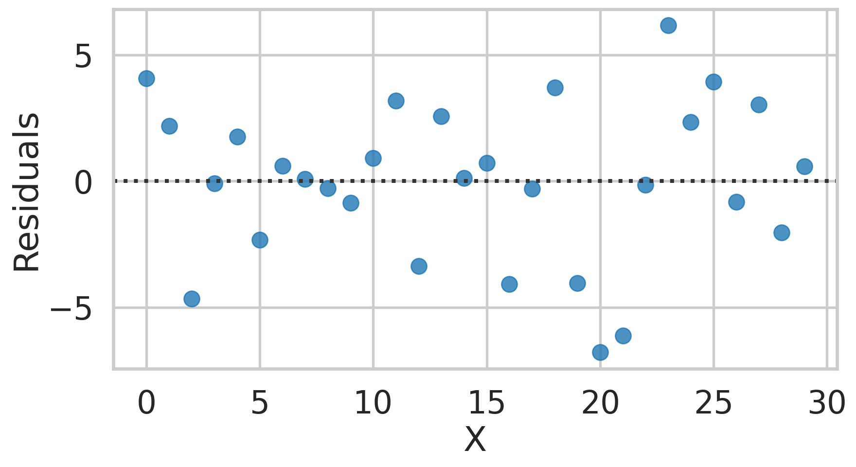
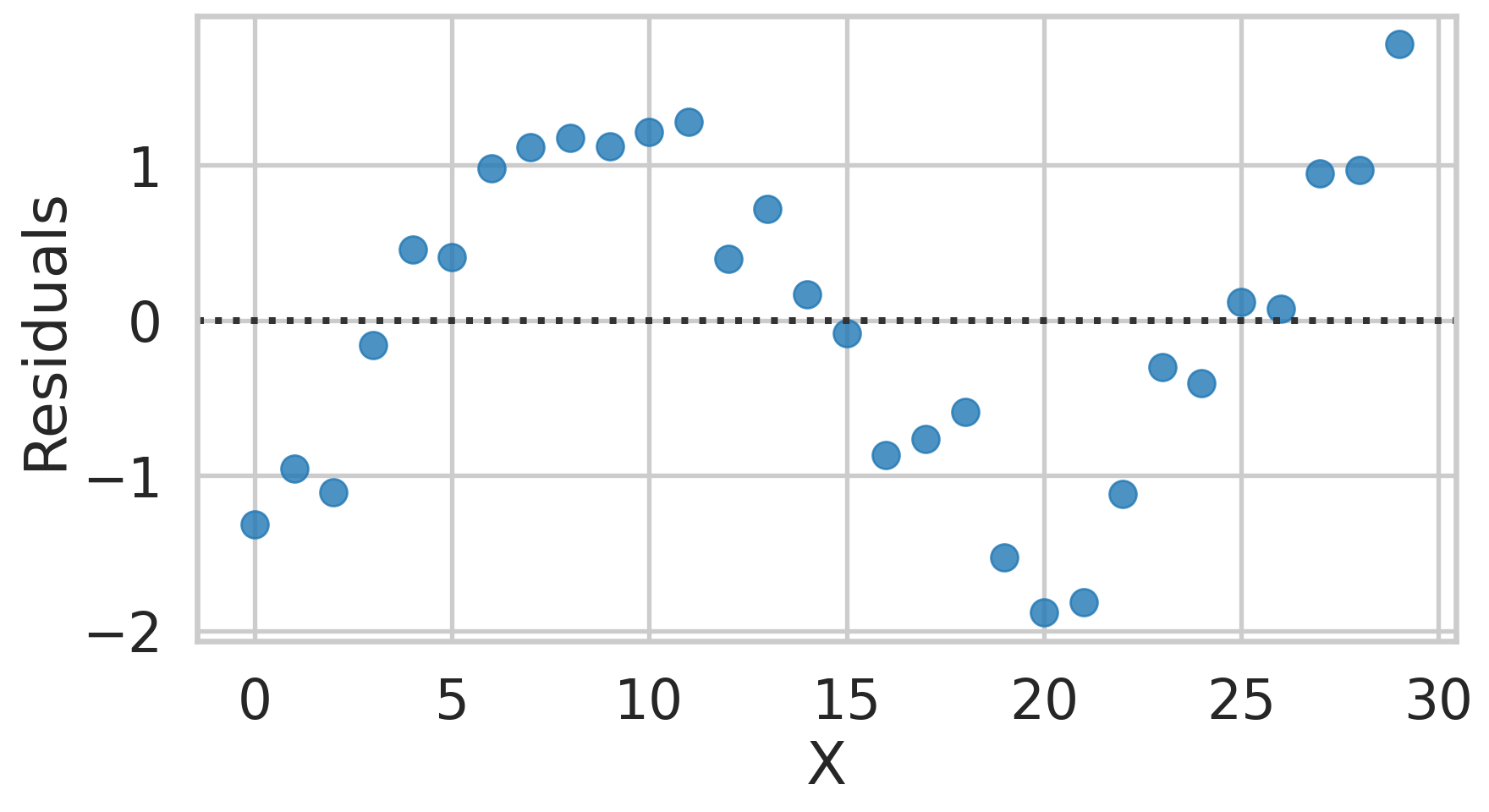
Residual Plot

Code

ax = sns.residplot(x=x,y=y)
ax.set_xlabel("X")
ax.set_ylabel("Residuals");

Independence of Error

The distances from the regression line to the points (residuals) should generally be random.
You do not want to see patterns
Was the previous plot of residual showing patterns, or was it more or less random?

Residual are independent?

Examples of Dependence

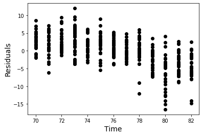
Time dependence can often be assessed by analyzing the scatter plot of residuals over time.
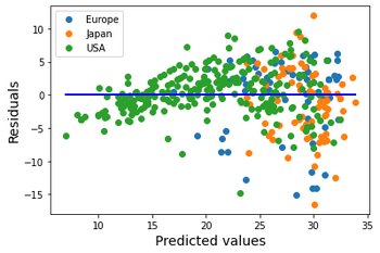
Spatial dependence can often be assessed by analyzing a map of where the data was collected along with further inspection of the residuals for spatial patterns.
Dependencies between observational units must be assessed in context of the study.

Example - Time

Example - Space

Discussion

In these graphs we saw time and spatial dependencies in our data set.
We saw this by plotting residual plots and looking for any patterns.
Recall the model was: \(MPG = m \cdot Weight + b\)
Does the independence of error assumption hold in this model?
Does that mean we should never use this model?

Mean and Variance of Error

Keeping error low and consistent

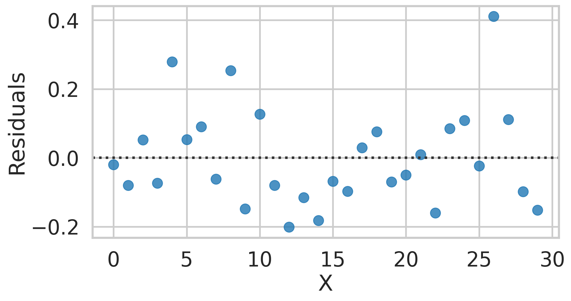
The residuals of a fitted linear model has a mean of 0. Always.
A mean of 0 means that on average the predicted value is equal to to the observed value.

Example, Residual 0

Example, Residual 1

Tip

Look at the y-axis scale!

Consistent Variance

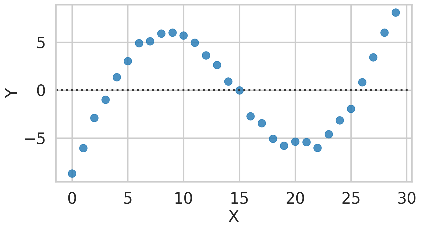
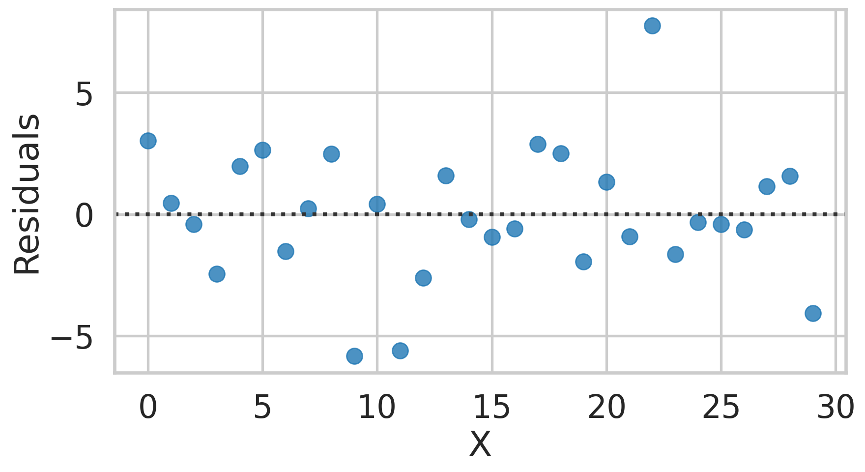
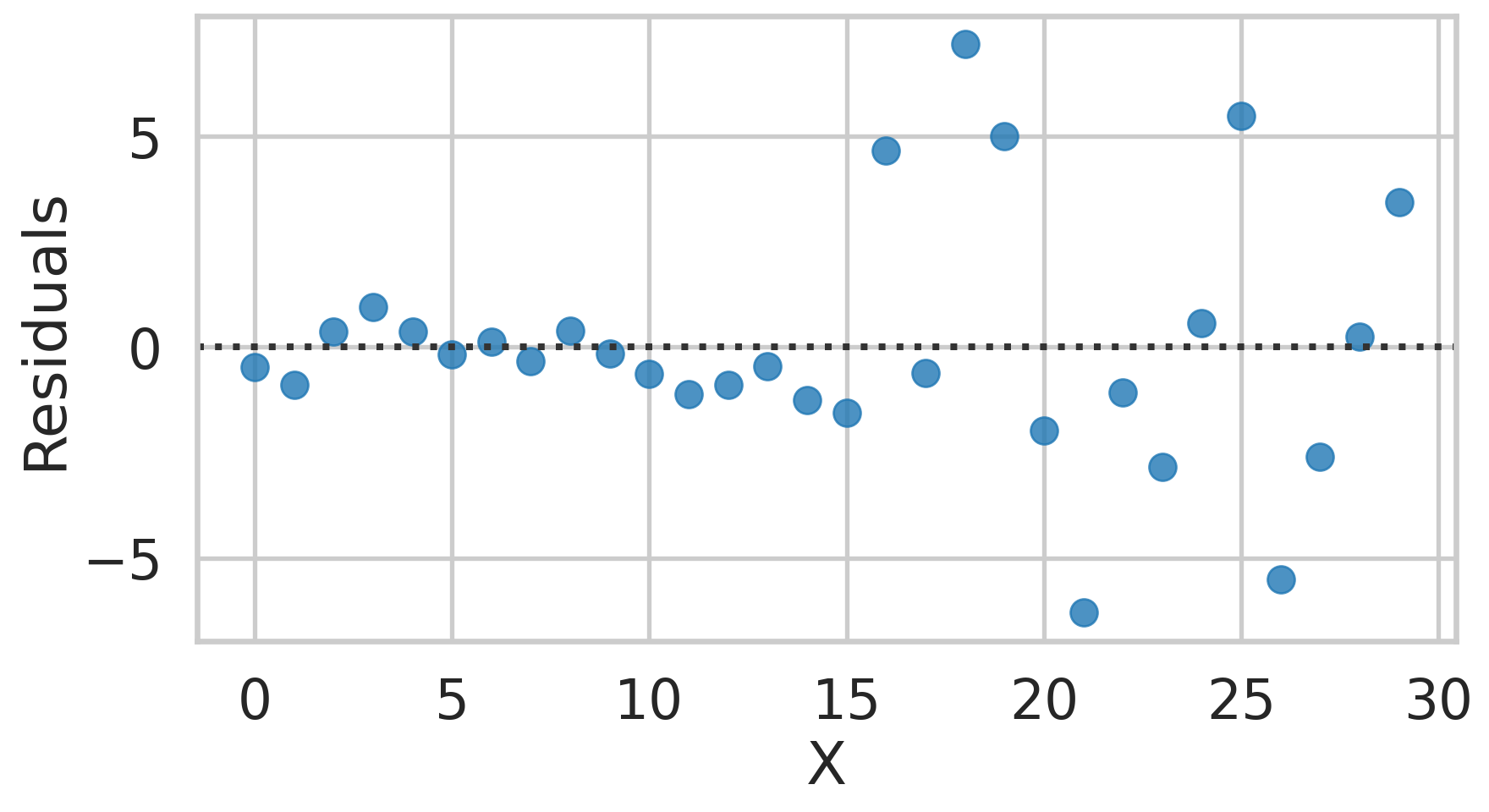
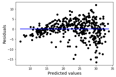
A linear regression should have a constant variance for all levels of the input.
That means the spread of the error should be the same at all levels of input
Level of input = x axis changing

Example, Residual 3

Example, Residual 4

Caution

Clearly see a huge jump in variance around 15

Example, MPG Prediction

Normality of Errors

As long as the previous assumptions hold you are going to get a good simple linear regression model
- \(x\) and \(y\) have a linear relationship
- Errors are independent (no spatial, time dependence, or other feature dependence)
- Residual mean of 0, variance constant
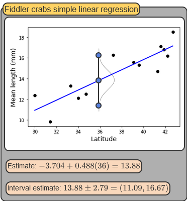
However, if the errors are also normally distributed, more awesomeness can be done: Interval Estimates

Interval Estimates

Full Example

Use library numpy and scikit-learn to fit our models
scikit-learn is library made for machine learning. Its awesome!

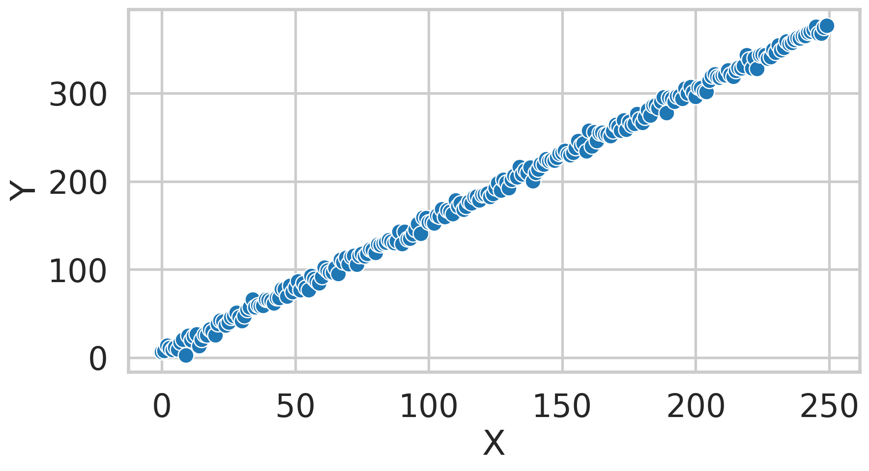
Creating data

n = 250
x = np.arange(n)
noise = np.random.normal(loc=0, scale=5, size=n)
y = (1.5 * x + 4) + noise
ax = sns.scatterplot(x=x,y=y);
ax.set_xlabel("X")
ax.set_ylabel("Y");

Creating data

Fitting the data

from sklearn.linear_model import LinearRegression
model = LinearRegression()

X = x[:, np.newaxis] # n X 1 matrix
reg = model.fit(X, y) # X needs to be a matrix

slope, intercept  = reg.coef_[0], reg.intercept_
print(f"Slope: {slope:.1f}; \nIntercept: {intercept:.1f}")

ax = sns.scatterplot(x=x, y=y)
ax.axline((0, intercept), slope=slope, color='r', label='Regressed Line');
ax.set_xlabel("X")
ax.set_ylabel("Y");

Fitting the data

Slope: 1.5; 
Intercept: 3.9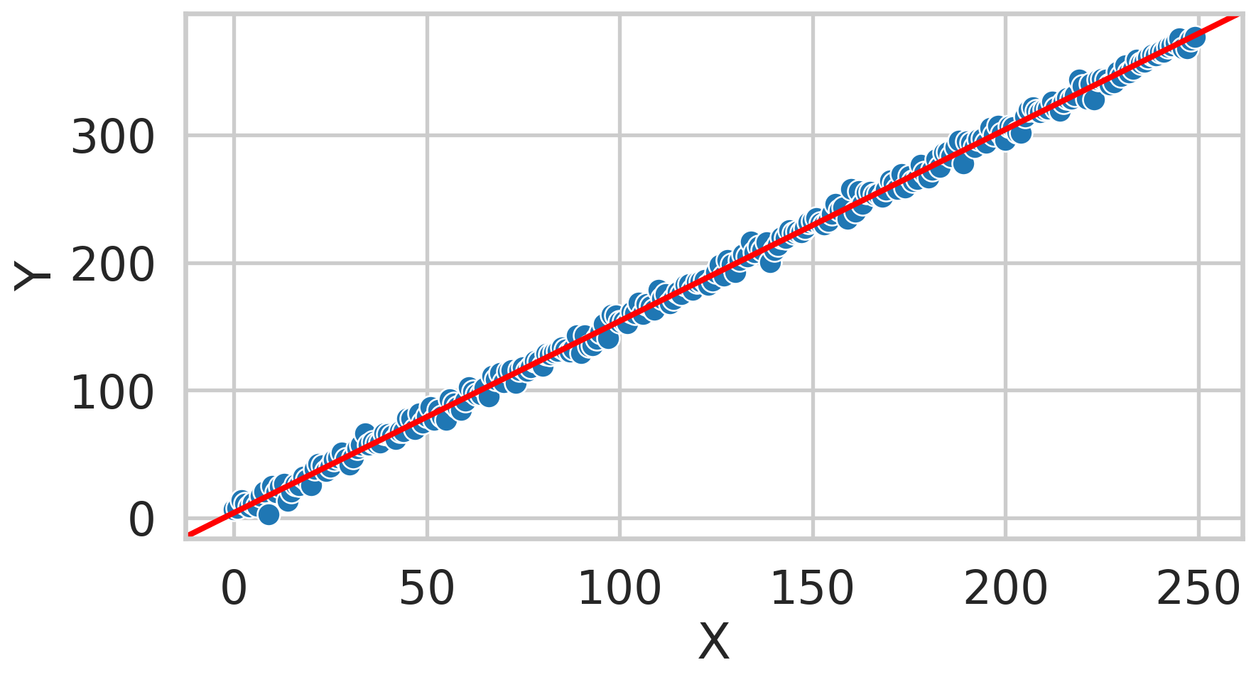

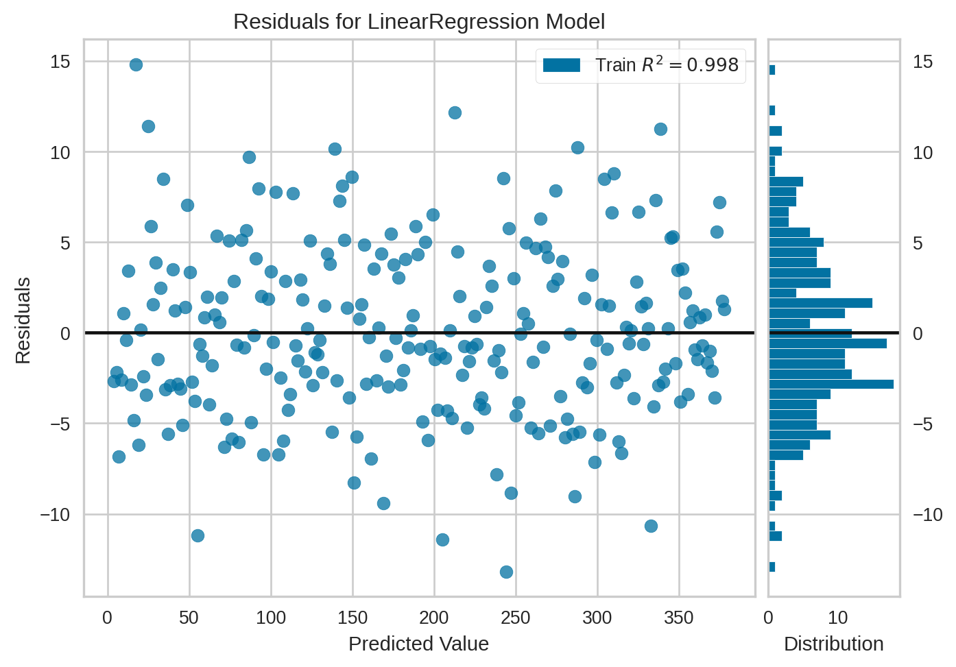
Residual Plot

from yellowbrick.regressor import ResidualsPlot
model = LinearRegression()
visualizer = ResidualsPlot(model)

visualizer.fit(X, y) 
visualizer.show();

Residual Plot

Multiple Linear Regression

Definition

Dataset has multiple input features
Incorporate more than one input feature into a single regression equation -> multiple linear regression
\(\hat{y} = \beta_0 + \beta_1 x_1 + ... \beta_k x_k\)
\(x_1, ..., x_k\) = input features
\(\hat{y}\) = predicted feature
\(\beta_0\) = y-intercept. \(\beta_1, ..., \beta_k\) = slopes

Example

pp = sns.pairplot(data=df,
                  height=7,
                  y_vars=['body_mass_g'],
                  x_vars=['bill_length_mm', 'flipper_length_mm'])

Example

3D plot

X = df[['bill_length_mm', 'flipper_length_mm']].values
y = df['body_mass_g'].values
def plot_plane(x_coef, y_coef, intercept, ax):
  x = np.linspace(X[:, 0].min(), X[:, 0].max(),  n)
  y = np.linspace(X[:, 1].min(), X[:, 1].max(), n)
  x, y = np.meshgrid(x, y)
  eq = x_coef * x + y_coef * y + intercept
  surface = ax.plot_surface(x, y, eq, color='red', alpha=0.5)

fig = plt.figure(figsize = (10, 7))
ax = plt.axes(projection ="3d")
ax.scatter(X[:, 0], X[:, 1], y, label='penguins')
ax.set_xlabel("Bill Length")
ax.set_ylabel("Flipper Length")
ax.set_zlabel("Body Mass")
ax.legend();

3D plot

Performing Regression

model = LinearRegression()
reg = model.fit(X, y) # X needs to be a matrix

slope_bill, slope_flipper, intercept  = reg.coef_[0], reg.coef_[1], reg.intercept_
print(f"Bill Slope: {slope:.1f}; Flipper Slope: {slope_flipper:.1f}; \nIntercept: {intercept:.1f}");

Bill Slope: 1.5; Flipper Slope: 48.9; 
Intercept: -5836.3

Visualize Plane

fig = plt.figure(figsize = (10, 7))
ax = plt.axes(projection ="3d")
ax.scatter(X[:, 0], X[:, 1], y, label='penguins')
ax.set_xlabel("Bill Length")
ax.set_ylabel("Flipper Length")
ax.set_zlabel("Body Mass")
plot_plane(slope_bill, slope_flipper, intercept, ax=ax)
ax.legend();

Visualize Plane

Simple Polynomial Regression

Special case of multiple linear regression
Include powers of a single features as inputs in the regression equation
Simple polynomial linear regression
\(\hat{y} = \beta_0 + \beta_1 x + \beta_2 x^2 .. \beta_k x^k\)
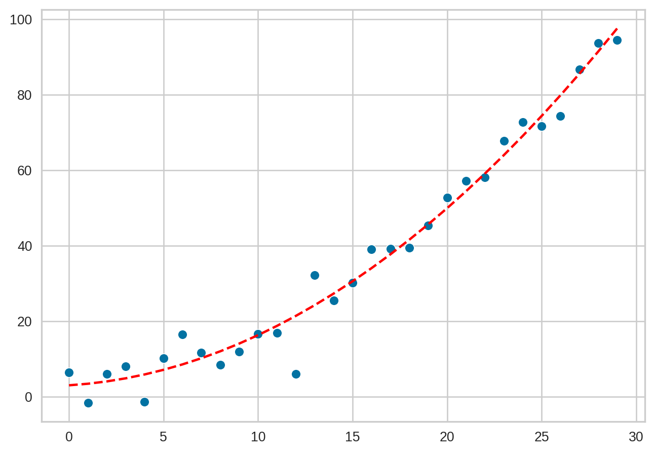
Quadratic: \(\hat{y} = \beta_0 + \beta_1 x + \beta_2 x^2\)

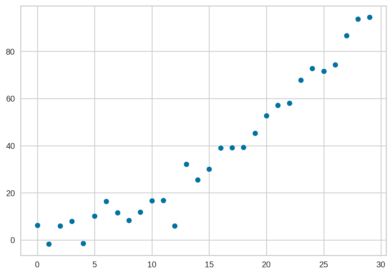
Example Quadratic

Code

n = 30
x = np.arange(n)
noise = np.random.normal(loc=0, scale=5, size=n)
y = (0.1 * x**2  + 0.3 * x + 4) + noise
sns.scatterplot(x=x,y=y);

Fitting a Quadratic (numpy)

coeffs = np.polyfit(x, y, deg=2)
print(coeffs); # beta_2, beta_1, beta_0

[0.1 0.3 3.0]

Plotting your regressed polynomial function

Code

regressed_fn = np.poly1d(coeffs)
y_hat = regressed_fn(x)
ax = sns.scatterplot(x=x,y=y)
ax.plot(x, y_hat, color='red', linestyle='--');

Fitting a Quadratic (SciKit Learn)

Scikit-learn can also fit polynomials
You must first create the additional columns manually
In other words create a second column that is the first column squared!
Helpful class called PolynomialFeatures

Fitting a Quadratic (SciKit Learn)

from sklearn.preprocessing import PolynomialFeatures
pf = PolynomialFeatures(degree=2,include_bias=False)
X = x[:, np.newaxis] # n X 1 matrix
x_features = pf.fit_transform(X)
print("Transformed Features:\n", x_features[:5, :])
model = LinearRegression()
reg = model.fit(x_features, y) # X needs to be a matrix
print("Coefficients")
print(reg.coef_, reg.intercept_); # beta_2, beta_1, beta_0

Transformed Features:
 [[0.0 0.0]
 [1.0 1.0]
 [2.0 4.0]
 [3.0 9.0]
 [4.0 16.0]]
Coefficients
[0.3 0.1] 2.965347007117529

Plotting your regressed polynomial function

Code

regressed_fn = np.poly1d(coeffs)
y_hat = reg.predict(x_features)
ax = sns.scatterplot(x=x,y=y)
ax.plot(x, y_hat, color='red', linestyle='--');

Class Activity

Practice Multiple Linear Regression